engineering
Learned Retrieval Weights: How Ditto Picks the Right Memories
We trained a lightweight MLP to dynamically weight semantic similarity, recency, and frequency signals for memory retrieval, achieving 98.8% intent accuracy with sub-millisecond inference.
On this page
Learned Retrieval Weights: How Ditto Picks the Right Memories
Most retrieval-augmented generation (RAG) systems rank memories by a single signal: semantic similarity. Embed the query, embed the documents, sort by cosine distance, done. This works well when every query is a topical search, but real conversations aren’t always topical searches.
When someone asks “what did we talk about yesterday?”, the best result isn’t the most semantically similar memory, it’s the most recent one. When they ask “what do I keep coming back to?”, neither similarity nor recency matters, discussion frequency does.
Fixed retrieval weights can’t adapt to these shifts in intent. We needed a system that learns to weight retrieval signals based on the query itself. This post describes how we built it.
Background and Motivation
Hybrid retrieval, combining multiple ranking signals, is well-established in information retrieval. The standard formulation blends sparse and dense scores with a fixed interpolation parameter [5]:
Recent work on Dynamic Alpha Tuning (DAT) [1] showed that dynamically adjusting per query using LLM inference significantly outperforms static tuning. Similarly, AutoMeta RAG [3] demonstrated that metadata-enriched retrieval achieves 82.5% precision compared to 73.3% for semantic-only methods, validating that auxiliary signals carry meaningful information.
Our setting extends this to three complementary signals in a personal memory system. Rather than using LLM inference (expensive, ~100ms per query), we train a lightweight MLP that predicts optimal weights in under 1 millisecond.
Problem Formulation
Given a user query and a candidate set of memory pairs retrieved via approximate nearest neighbors (HNSW [12]), we compute a composite score for each candidate:
where are query-dependent weights satisfying , and the three scoring functions are:
Cosine similarity : Semantic relevance between the query embedding and memory embedding, computed via pgvector [12]:
Recency : Temporal proximity, normalized across the candidate set. Following research on freshness-aware ranking [4, 6], we use linear decay:
where is the timestamp of pair , and are the oldest and newest timestamps in the candidate set. This relative normalization means “recent” adapts to the time span of retrieved candidates.
Discussion frequency : How often the memory’s topics appear in conversation, derived from subject-memory link counts in our knowledge graph:
The key question: how do we predict optimal from the query alone?
Neural Architecture
Inspired by entropy-based hybrid retrieval [7] and attention fusion approaches [2], we use a Multi-Layer Perceptron with auxiliary feature inputs. The architecture processes the query through two paths that are fused before the final prediction:
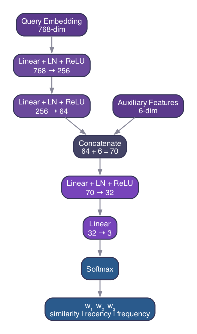
Embedding path. The 768-dimensional query embedding (from Google text-embedding-005 [13]) is projected through two fully-connected layers with layer normalization and ReLU activation:
Auxiliary features. Embeddings capture semantics but can miss explicit lexical cues. We extract 6 handcrafted features from the raw query text: normalized query length, binary temporal keyword detection, binary frequency keyword detection, temporal keyword density, frequency keyword density, and a specificity indicator for named entities. These features are cheap to compute (keyword matching only) and provide strong signal that embeddings alone would miss.
Fusion. The embedding representation and auxiliary features are concatenated and projected to the output:
The softmax output guarantees with all weights non-negative. The full model has approximately 216K parameters (~845 KB), small enough to embed directly in the application binary.
Training
Synthetic Data Generation
Collecting labeled retrieval preference data from real users raises privacy concerns and requires significant interaction volume. Following recent work showing that LLM-generated synthetic queries can rival human-written queries in training utility [8, 9], we use an LLM to generate 1,000 diverse query-weight pairs across four intent categories:
| Intent | Example Query | Target Weights |
|---|---|---|
| Semantic | ”Tell me about my Python projects” | |
| Temporal | ”What did we discuss yesterday?” | |
| Frequency | ”What topic keeps coming up?” | |
| Mixed | ”Recent updates on that ongoing project” |
Each generated example undergoes self-consistency validation: the dominant weight must align with the stated intent category. Queries are embedded using Google text-embedding-005 [13], and auxiliary features are extracted to form the complete training tuple .
Loss Function
We use a multi-task objective combining distributional matching with entropy regularization, inspired by cross-encoder distillation approaches [8, 10]:
The primary term is KL divergence between predicted and target weight distributions:
The entropy regularization term () penalizes low-entropy predictions to prevent mode collapse, ensuring the model doesn’t degenerate to always placing all weight on a single signal:
Results
Training with AdamW (, weight decay ) and cosine annealing over 25 epochs:
| Metric | Value |
|---|---|
| Test KL divergence | 0.025 |
| Weight MAE | 0.053 (±5.3% per weight) |
| Intent classification accuracy | 98.8% |
| Training convergence | ~15 epochs |
The 98.8% intent accuracy means the model correctly identifies the dominant retrieval signal (semantic, temporal, or frequency) in nearly all cases. The low weight MAE indicates it also produces well-calibrated blends for ambiguous queries.
Deployment: Pure Go Inference
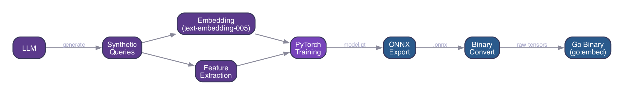
A critical design decision: we run inference as pure Go math embedded in the backend binary. No Python sidecar, no ONNX runtime, no external service.
The deployment pipeline:
- Train in PyTorch (standard ML workflow)
- Export to ONNX for standardized tensor representation
- Convert ONNX to a compact binary format (raw tensors with shapes)
- Embed in the Go binary via
//go:embeddirective
The Go forward pass implements linear layers, layer normalization, ReLU, and numerically stable softmax from scratch, roughly 200 lines of pure arithmetic. The model loads once at startup via sync.Once. Each prediction takes ~0.5–1ms with zero allocations that survive the request.
If the model fails to load for any reason, we fall back silently to default weights . Zero-downtime, zero-config.
Why not a remote service? Latency and operational simplicity. An embedded model means zero cold starts, zero network hops, and zero service mesh complexity. The tradeoff is that retraining requires a binary recompile, acceptable for a model that doesn’t need daily updates.
Composite SQL Retrieval
With predicted weights in hand, all three signals are computed and combined in a single SQL query against Supabase (PostgreSQL + pgvector [12]):
- HNSW retrieval: 50 approximate nearest neighbor candidates via pgvector
- Frequency scoring: Aggregate subject link counts from the knowledge graph
- Recency normalization: Relative to the candidate set’s time span
- Composite ranking: , returning the top
One database round-trip. All scoring is atomic in SQL, no application-level re-ranking.
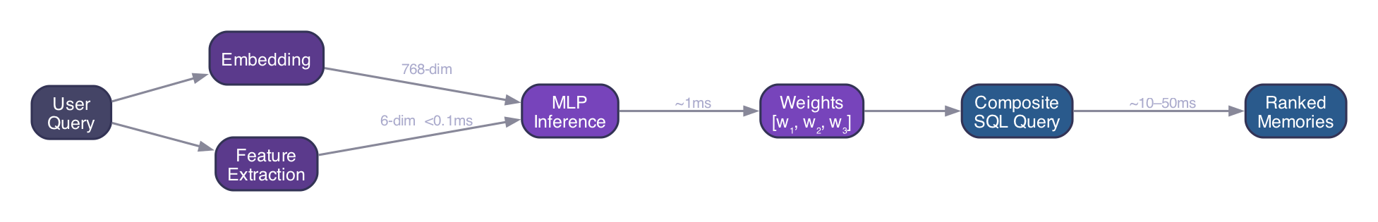
End-to-End Latency
| Stage | Latency | Notes |
|---|---|---|
| Feature extraction | <0.1ms | Keyword matching in Go |
| MLP inference | ~1ms | Pure math, no allocations |
| Composite SQL query | ~10–50ms | Single CTE with HNSW |
| Memory content fetch | ~50–200ms | Parallel Firestore reads |
| Learned weights overhead | ~1ms | Negligible vs. total |
The learned weights add approximately 1ms to the retrieval pipeline. The dominant cost remains I/O (database and Firestore), which is unchanged.
User-Facing Transparency
We believe retrieval decisions should be inspectable. In the Ditto app, expanding the seed memories panel on any message reveals:
- Predicted weights: The percentages the model chose for that query
- Predicted intent: Whether the query was classified as semantic, temporal, or frequency-oriented
- Per-memory scores: Color-coded bars showing each memory’s similarity (blue), recency (amber), and frequency (emerald) contributions
- Composite score: The final weighted score as a percentage
This transparency lets users understand why Ditto surfaced specific memories, building trust in the retrieval system.
Impact on User Experience
With learned weights handling retrieval quality automatically, we simplified the product:
- Removed long-term memory configuration: Users no longer need to tune tree depth or branching factors. The system optimizes automatically.
- Removed the memory paywall: All users now get the same high-quality retrieval. Memory is core to the product, not a premium feature.
- Retained short-term memory control: The one setting users intuitively understand (how many recent turns to include) remains adjustable.
Future Directions
Online learning. The architecture is designed for per-user adaptation. The current global model could be fine-tuned on implicit feedback, did the user engage with retrieved memories?, to produce personalized weight vectors over time.
Alternative decay functions. Our recency score uses linear decay; research suggests Gaussian () and exponential () decay [6] may better capture different temporal preferences. These could be learned jointly or selected per query.
Attention-based fusion. Inspired by Fusion-in-T5 [2], a cross-attention architecture over learnable signal descriptors could provide more interpretable weight predictions with per-result granularity rather than per-query weights.
Human preference data. As Syntriever [9] demonstrates, partial Plackett-Luce ranking models can learn effectively from implicit preference signals. Combining our synthetic pre-training with real user feedback is a natural next step.
A tiny neural network, embedded in a Go binary, making sub-millisecond decisions that meaningfully improve every conversation. No external services, no infrastructure overhead, no knobs for users to fiddle with. It just works.
- Omar
References
[1] DAT: Dynamic Alpha Tuning for Hybrid Retrieval in RAG. arXiv, 2025. arxiv.org/abs/2503.23013
[2] Fusion-in-T5: Unifying Variant Signals for Simple and Effective Document Ranking. ACL, 2024. aclanthology.org/2024.lrec-main.667
[3] AutoMeta RAG: Enhancing Data Retrieval with Dynamic Metadata-Driven RAG Framework. arXiv, 2025. arxiv.org/abs/2512.05411
[4] Learning to Rank for Freshness and Relevance. Microsoft Research. microsoft.com/en-us/research/publication/learning-to-rank-for-freshness-and-relevance
[5] Hybrid Retrieval for Enterprise RAG. 2024. ragaboutit.com/hybrid-retrieval-for-enterprise-rag
[6] Time-based Ranking in Milvus. Milvus Documentation, 2024. milvus.io/docs/tutorial-implement-a-time-based-ranking-in-milvus.md
[7] Entropy-Based Dynamic Hybrid Retrieval. OpenReview, 2024.
[8] Teaching Dense Retrieval Models to Specialize with Listwise Distillation and LLM Data Augmentation. arXiv, 2025. arxiv.org/abs/2502.19712
[9] Syntriever: How to Train Your Retriever with Synthetic Data from LLMs. NAACL, 2025. aclanthology.org/2025.findings-naacl.136
[10] Enhancing Transformer-Based Rerankers with Synthetic Data and LLM-Based Supervision. RANLP, 2025. aclanthology.org/2025.ranlp-1.109
[11] Mixture of Logits (MoL): Efficient Retrieval with Learned Similarities. WWW, 2025. arxiv.org/abs/2407.15462
[12] pgvector: Open-source vector similarity search for PostgreSQL. github.com/pgvector/pgvector
[13] Google text-embedding-005. Vertex AI Documentation. cloud.google.com/vertex-ai/generative-ai/docs/embeddings/get-text-embeddings
Open a thread.
Ditto remembers what matters from every conversation, so your next idea starts where your last one left off.